Wolfram Student Podcast S2 Ep 8: Evaluating Complexity for Neural Nets in Learning Math Functions
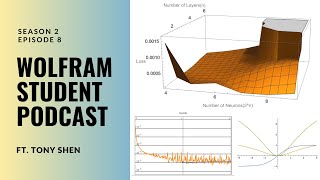
Tony investigated how neural network size affects learning math functions. He varied neurons from 1 to 1,024 and layers from 3 to 8, finding a U-shaped pattern where performance improved to an optimal point, then got noisier with larger networks. Computational limits prevented more training rounds.
Chapters
Hello, everyone, and welcome to season two, episode eight of the Wolfram Student Podcast. I'm Sam.
And I'm Roshank.
And we're your hosts.
This is the Wolfram Student Podcast, where every fortnight we dive into a new innovative project done by high schoolers using the Wolfram language.
For this episode, let's welcome Tony, who'll be discussing his Wolfram summer research project on evaluating the impact of complexity, variation and neural nets on learning math functions. Hi, Tony.
Hello, Sam. My name is Tony. I'm from Newport High School in Bellevue, Washington. I'm a current junior and I attended the Wolfram Summit research program in 2023.
Yeah, sounds really cool. Did you have any experience with Wolfram before you had come to the summer research program, or was this your first time?
This is actually my first time using the Wolfram language. So, yeah, it was a pretty interesting experience for me.
Cool. Yeah, I mean, hopefully I had a great time at the summer camp and learned a lot about it. And just a fun question we like to ask everyone who comes on the podcast. What's your favorite Wolfram function?
My favorite Wolfram function, I would say, is the net chain function. So is basically this one function that kind of take in parameters for your neural nets for the data and training rounds, validation sets and everything. And you can call this function to include all those inputs and then actually train the neural nets. And this function also provides you with a visual graphics of where the loss functions looks like per round of training. So that's really, really cool comparing to when I'm doing machine learning projects with other languages like Python. In Python, it's simply like a black box. When you're training the neural nets, you don't actually see what's going on. But this net chain function, it visually presents you the loss as the training goes on. So that's really, really cool for me.
Yeah, no, that sounds pretty cool. Notice that people generally go with like either project specific functions like netchain, I think, or a more general function like table that's like pliable everywhere. So, yeah, I think it's cool to see how just how people's ideas of their favorite functions change based on what project they get into. Anyway, so let's just get into your project. Before we start, can you give me like a quick summary of what it's about?
So my project focuses on machine learning and with some sort of. With some level of math involvements within it. My project aims to answer the question, to what extent does varying the complexity of neural networks affect the efficiency in Learning mathematical functions and, and how can these changes be quantitatively measured? So this project aims to investigate the relationship between the complexity variation of neural networks and how well they learn different mathematical functions, while creating this new methodologies of quantitatively measuring how well the neural networks learn.
Yeah, okay, that sounds really cool. Cool. Do you want to just dive right in?
Yeah. So yeah, a few keywords before going into my project. Neural networks is a model built with many nodes and they work together to process information. And in my project specifically, they're working together to learn how a mathematical functions works and how it would look like according to different data points. And activation function is just this like initial function that the neural networks is running on before learning the data points. And the loss refers to the difference between the model's prediction and the actual input. So it represents the precision of the neural networks in learning the inputs. So in order to quantitatively measure how well a neural networks learn different mathematical functions, we need to develop some sort of criteria. Right. So here in my project, the first criteria that I developed is the amount of neurons in the neural networks. So by varying the amount of neurons in neural networks, I kind of expect to see different level of losses which the neural networks will result. So that will kind of show me what will be the most optimized amount of neurons that a neural networks will require in learning a specific mathematical functions. So here to get started, we have this function right here, E to the power of negative absolute of x plus absolute of Y squared. So it's pretty complex. We're using this function to like kind of find a very, very hard function to model on. So yeah, we're just using this as an example to train some neural networks and see how well they perform. So here I have this function and I took out some data points from this function in the interval from X Y negative 3 to positive 3. And I took these data points. First I pull out a neural networks of 32 neurons serving function tangent H. And then I'm training these neural networks on the, on this mathematical functions. Right. So here you can see the results. The loss is pretty significant and we're training two rounds on this. So from here we can actually like pull out some really, really important properties that we can use to analyze the efficiencies and complexities. The loss for sure. Also just the rates which the loss decreases. Right. So how well does the loss improve with according to the training routes? So here we're using these two ideas and we're training this group of data that we generated earlier with mathematical Functions on different neural networks with different amount of neurons. So here I varied the neural networks from 2 to the power of 0, which is 1 neuron, to 2 to the power of 10 neurons, which is 10, 24. Okay, so the.
Sorry, one question if you scroll up to that graph there, just to be clear, is a higher loss is bad, right? So by the end of round two, the loss was better, as in you weren't losing a lot of precision.
So what this loss represents is representing the difference between the. The result from the neural networks and actually inputs. Right. So at the beginning of the training, you can see that the loss is very high, which means that the difference between the result from the neural networks and the actual inputs is very high. So that means the neural networks is not precise in estimating the mathematical function. And after two rounds of training, the loss became smaller than 10 to the power of negative 4, which is a small loss. So that means that the difference between the prediction from the model and the actual results became closer after two rounds of training.
And that means the more rounds you did, the, the closer that the training data approached the validation set, Right?
Yeah, yeah, you can take it that way. And yeah, but here we. Yeah, here's also a limitation from my project. Because of the limits in the computation power I have, usually the training rounds should go for more rounds, maybe eight rounds. Ish. But I had very limited computational power and I was only able to run two rounds on my data. So this is a limitation on my project of how accurately like these neural networks are actually like representing the mathematical function.
Yeah, okay, thank you.
But, yeah, so, yeah, so what I did here is I buried in neural networks with 10 different amount of neurons. So for example, with 1, which we see with 1 neurons of this neural networks is giving out a loss function that's really, really high comparing to the one we did before, which is 32 neurons. And we can kind of observe this pattern with the variation of neurons that the loss was in generally decreasing. So with 2, 4, 8, we can see that the loss function is getting lower and lower and the precision and accuracy are increasing as we increase the number of neurons. But here I also made a pretty interesting observation that if I increase the neurons to a very high amount, for example 512, which is to the power of nine, and when we have this huge number of neurons modeling a mathematical functions, we see that there are a very absurd amount of noises in the loss function. So this is actually represents an increase, an improvement in the accuracy or a decreasing in accuracy. So that's another thing that I kind of like when, that I kind of investigated in my project. So here just putting all the graphs together from 1 to, from 2 to the power of 1 to 2 to the power of 10, we have these 10 graphs and we can observe the general trends that I just explained. The loss generally decreases and after a certain point the noises of the loss functions became very significant. And we can see that the validation sets for 2 to 10 neurons especially is presenting a pretty significant differences between the training data and the validation data. So these are like the outliers that I want to eliminate in analyzing what will be the most optimized number of neurons to train a mathematical function. So here's the first criteria of varying a different number of neurons in analyzing the accuracy. So yeah, here's also a plot that I kind of pull out. So on the x axis you have the different number of neurons in your networks and on the Y axis you have the loss function, the accuracy between the predicted value and actual values. We can kind of see this quadratic function presented in, in the graph. And that means there has to be like one point that's neither too little neurons or too much neurons. There has to be one point with a like really, really, I guess like lucky number of neurons that kind of provides you the highest precision in estimating the mathematical functions. So this is what I later called an optimization point. And this is the point that we want to find for a series of neural networks that approximate for a mathematical function. So we want to take out this one fixed point in analyzing how complex the mathematical function is. So yeah, that was the first criteria. And the second criteria is the number of layers. And yeah, similarly we have an example functions, we pull out many data points of that example functions on this negative 3 to 3 range and domain. And we applied the similar methodologies which we varied the amount of linear layers in the neural networks and then we observed the changes in the, in the loss. So for loss functions, I for the different number of layers variations, I vary them from three layers to eight layers. And this number came from the testings that I've done with different amount of linear layers in the neural networks. If there's only one layer or two layers, they, they don't usually perform well. So they're the outliers that I eliminated in the analysis. And here we're putting the loss functions from these different layers together to kind of analyze their position. So you can also see this general trends that if we have more layers, the precision generally improve. The loss function generally decreases. But as we increase the layers above a certain threshold, the loss function also like incorporate this very significant noise that actually decreases the precision of the, of the neural networks. And here similarly with the variations in neurons, we're putting the variations of layers together and we can also kind of see this quadratic like functions. And we're also aiming to pull out this optimization point from the layers variations of a neural network.
So you're essentially saying that for both number of layers and number of neurons, there's like a Goldilocks kind of point where loss reaches its minimum. Do you have any ideas about like why it doesn't, why there is an optimization point and it doesn't like always decrease or always increase in a sense.
So there is definitely some mathematical reasoning behind that. I believe the term for it is back propagation. So an example of such ideas will be if we just have a linear function of Y equals to X. Right. So the math data points that we're pulling out of this function is basically like 000-505-11. So there is this really not complex, direct intuitive relations between the data points. And in this case, if we incorporate a huge number of neurons and layers, that means we're creating a very, very complex neural networks. And as we input the data points into one neurons, whatever is in that neurons, the weights will be sent to like 10 more neurons and probably like 100 more neurons, which create a very significant noise in the estimation that the neural networks produce. So the more in depth analysis of how back propagations relates to why this optimization point exists and the exact math relations between where to find this optimization point, that's a future work which I want to conduct with this project. But I don't currently have an rational answer to, to back up with my observation here.
Yeah, no worries. Okay, thank you so much for explaining.
Yeah. So, yeah, following the development of these two criterias, the layers variations and neuron variations, what I did here essentially is that I'm abstracting the algorithms, abstracting all my code together so that I have this one function that when I input the math functions into this one programming function, it will provide me the optimization points. So here we generate the data, we train nets with variations of neurons, between nets with variations with layers, and then we put it together, we find the most optimization point. So here's the attraction of the algorithms. And after this step, what I did is that I kind of pull out the loss functions of each number of neurons and each number of layers and I constructed this 3D graph of what the loss functions look like with regards to these different variations. So here we can see like a valley, like CBD graph. So this is like a more intuitive way to observe how well the variations in layers and neurons will perform as we change them. And we can more intuitively find this optimization point that we are looking for in analyzing the complexity of a math function. So, so here, yeah, op point, optimization point, we're pulling that out. Number of neurons to power seven and number of layers, one layer. And here's the loss function, the accuracy or precision that the neural networks has. And right here, this is the one function that I call so to train on all these neural networks and produce the optimization point. So that kind of leads into the analysis stage. So my purpose in the analysis stage is that I want to run my model through a wide variety of math functions. Linear functions, quadratic functions, cubic functions, trig functions, logarithmic functions. So yes, so as you can see here, I did train a lot of neural networks and pull out the optimization points for those. And I want to graph of these points into like one Cartesian planes so that the functions with that are generally less complex. I'm expecting to see a low number of neurons and layers. For the functions that are more generally complex, I'm aiming to see a higher number of neurons and layers. So there will be this distinction graphically between how to distinguish a less complex math function and a more complex math functions. But unfortunately here I wasn't able to really pull out a precise graph because of the limitation of computing power I mentioned earlier. I figured that the loss functions here in the analysis stage were kind of imprecise because I only trained them for two rounds. So for some of the functions like this polynomial, you can see that the loss is 0.13, which is very, very, very high. And for this logarithm function, you can see that the optimization point is 0.00001. So I wasn't able to really pull out this. I wasn't able to make the functions all to a fixed number of preciseness. So there are some neural networks that are very imprecise and some neural networks that are pretty precise. And of course, the result of comparing those neural networks would not be very persuasive in explaining the complexity. So that's the limitation that I had that didn't lead to a very good answer. Yeah, so, but, so you can see that the graph of these complexity of neural networks results in this kind of logarithmic curve that we have. So, yeah, why this pattern exactly emerge is also like Another thing that want to work on in the future here, just comparisons of the functions, activation functions and some trig functions. And yeah, I want to do an investigation of how the backpropagations kind of relates to these differences and how they affect the neural networks. But I didn't get enough time to work on those during my summer project, during the summer camp. And yeah, those are the future works that my projects kind of lead to. So conclusion, this new approach, this new methodologies of understanding the complexity of mathematical function is pretty intriguing and also it's a pretty reliable way to analyze the complexity of math functions. Assuming that we have enough computing power, we have this evaluation matrix from different number of neurons and different number of layers, then we can find the most optimized point and we can use that as a helpful tool to evaluate the complexity of math functions. However, with the limitation that I brought us before, I did not have enough computing power unfortunately. And also all of my neural networks here in this project are trained on the same activation function. It's a parabolic tangent function. And that might have something to do with how the loss functions perform as we vary layers and neurons. And as well there is some limitations when I'm generating the training data. So the functions, for example, the function has to be continuous over the interval otherwise it'll produce some really like absurd patterns and also undefined points that my networks cannot take account of. So yeah, of those I want to put them into sort of like the future works of my project to relate the mathematical back propagations to interpolate data which is putting all the variations into a more like a, like a 3D graph but with a smoother curve so that I can truly find where the optimization point is. Right now is kind of chunky. So I'm finding this. So for example, here I'm finding this point as the lower point. But if I interpolate the data, the quadratic function will become smoother and maybe the most optimized points will be in between four and five. So that could also further help me to analyze the complexity. And yeah, definitely more data is into like more functions, more math functions should be inputted into the model so that we can have a more precise representation of where their complexity lies on the XY graph of different number of neurons and different number of layers. Yeah, so that's the conclusion of my project and I want to acknowledge my mentor Eric and also a special thanks to Nicole with all his help and suggestions during my project.
Yeah, this is really cool. Thank you so much for showing everything and exciting the saw then. Yeah. Before we end, I know you talked about some of your limitations of this model and some things that you wanted to improve with it, but beyond just this project, is there anything beyond that that you'd like to do with the Wolfram language?
So Wolfram language has this really nice connection to the Wolfram database, and it has a lot of functions to visualize the data. So I'm actually looking forward to use Wolfram language as a helpful tool in creating some video tutorials for the math classes in my school. So I observed that some of my fellows and my classmates, they're struggling on understanding some of the concepts in calculus. And I want to use both from language and its power to visualize to kind of create like, tutorials for them to better understand what's going on behind the math, behind the numbers.
Yeah, that sounds really cool. Okay. Wish you best of luck, you know, to work on that project and anything future you want to do with orphan language. If you ever create something cool, you're always welcome to come back on the podcast. Yeah. Thank you so much for coming and it was great to hear from you.
Yeah. Thank you. Thanks for listening to this episode of the Wolfram Student Podcast. We hope you learned something new and took away insights from today's discussion. If you want to be featured in a future episode, fill out the form@tinyurl.com WSP S2 interest and be sure to.
Tune back in two weeks time to hear our next episode. Once again, thanks for listening to this episode of the Wolfram Student Podcast.
More from Guy


Cheryl Strauss Einhorn | The Human Edge: Smarter Decisions in the Age of AI | Talks at Google



Rachel Glennerster | Innovation and the Center for Global Development | Talks at Google

Rebecca Winthrop | Rethinking the Purpose of Education in the Age of AI | Talks at Google

Dr. Robert Wachter | A Giant Leap: How AI Is Transforming Healthcare... | Talks at Google



