TS4 / XIII-03: AI for forcasting DH demand and fault detection
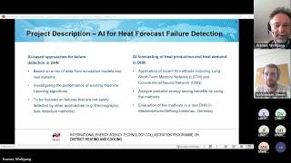
Wolfgang, Simon Goldshauser, and Mathieu Vallier present an IEA-funded project using AI to forecast heat demand and detect faults in district heating networks. A CNN model achieved 4.2% mean absolute error on a 12-hour forecast. Implementation costs around €25,000–30,000 could yield €10,000–20,000 in annual savings from avoided overheating.
Questions this video answers
Approximately one year of data at 15‑minute sampling rate (Meckenberg, Germany).
An autoregressive convolutional neural network (CNN) was used as the best-working model, though LSTM and other models showed nearly equal performance.
Mean absolute error 4.2% with respect to the maximum Q̇ occurring during the year of data.
80% CI: −7% to +7%; 90% CI: −9% to +10% (relative error ranges).
12 steps of 1 hour each → 12 hours ahead (multi-step forecasting).
Chapters
But everybody should see my screen now. Is that okay?
Yes, perfect.
So, welcome back after lunchtime for our presentation. Here my colleagues and I will present the IEA funded DHC project. Artificial Intelligence for Fillet Detection Forecasting of Heat Production, Heat demand in district heating networks. And once more the reminder concerning the recording. We don't need this anymore.
Maybe I just start with showing the project partners.
On the one hand side is our institute Fraunhofer Ise in Germany, concerning the forecasting heat demand. The other part is done by ca. The well known ca, Lytton, Matthien Vallier will present their part on the fault detection. And the person you probably don't know is Michael Steiber, who is head of the operation of the Realistic Heating network in Lebanon. They run a small district heating network where we use data for putting up or mounting up the methods and also for the evaluation.
And Simon Goethe is here with us. He's going to present the part on the heat forecasting with AI. I am doing a very short introduction right now and talking about the two parts or two topics which have been touched in this project. One is on the failure detection, as the title already shows, and the other one is on heat demand. And both approaches, or both topics are using AI methods. The failure detection part was looking into a modeling of holes with simulation models of components of the dhn. They, the colleagues of CI were looking into the performance of machine learning algorithms and they focused on failures which are not easily detected by other approaches like thermography or lead detection. Because in these cases obviously the special benefit can be created on the part of the forecasting. We analyzed several different methods of AI for forecasting, like the short term memory network approach LSTM and the convolutional neural network cnn and also an older approach on ANN and LSI combination.
We analyzed the potential of energy savings benefits by using these methods in the real network in Libeno. And obviously we did also the evaluation of the methods in the real district heating network in Libenau. So now I hand over to Simon.
Your turn.
Yes, thank you.
Just let me see. Sorry, no.
Okay, so this is where my path starts. I'm Simon Goldshauser, I'm with the ESA now for two weeks full time. And before I worked on this topic as a student researcher. Yes, so the prediction of the future heat demand in the DHN we wanted to do on the one hand for single consumers and also then for the total network, as Wolfgang already said, with artificial neural networks, with the goal in the end to provide supportive information for the network operation, which can on the one hand be for a human operator and in further steps maybe also for an automatic operation of the whole network.
The data that we use to train, validate and test the models, as Wolfgang has already said, was recorded.
In Meckenberg in Germany. And we had roughly about one year of data at sampling rate of 15 minutes, which includes supply and return temperatures, flow rates, power and pressure meter readings for different buildings.
Which also includes weather data and also weather forecast data from the online service Meetup Blue.
Here you can see how the data looked like when it was inputted into the networks and also what the output then would be. So we have our current time step t, so the current time from which one we want to predict here.
And.
From the past time horizon we input the past heat demand of the network. And for weather information, ambient temperature and global horizontal irradiance related with some temporal context that should catch some temporal reoccurring patterns or stuff like that. And for the weather data we also have a future forecast for ambient temperature and global horizontal irradiance that is also added as more context information for the future part of the heat demand that we want to predict. Also in combination with the temporal context information.
We evaluated two different multi step prediction approaches as we wanted to predict not only one time step into the future, but several time steps. We can do that by a single shot approach where we predict everything at once, so all the input goes in into the model and all output time steps come out at once. And we can also use the autoregressive approach where we predict step by step. So we do one time step prediction and we use this prediction for the next one and for the next one and so on.
As Wolfgang already said, we checked out two network architectures where one of them is the convolutional neural network. This is a network that is mainly used in image processing tasks as it applies something like 2D filters to data in its so called convolutional layers. This is a little bit depicted at the bottom. So you see here like this short purple rectangle that is 2D filter on the input data, creates new data point in the next layer and so on and so on, and in the end we get the final output. On the other hand, we looked at the long short term memory networks which is one that is especially made for processing sequential data as it has recurren connections and can by that recurring connections maintain something like an internal state. So it has some kind of.
Memory as the name suggests, and it's mainly used in natural language processing tasks, on the bottom here you can see. Oh, sorry.
Yeah, maybe just back. So I have say a few words for the architecture. You have the input, then the network where we have this recurrent connection and final output layer creates the output. When you unfold this over time, you have something like the picture on the right where you have the same LSTM network over and over again and the recurring connection hands over its internal state to the next prediction step. Okay, now.
Next slide. Thank you.
Coming to the results, what we then did in the end is prediction of 12 steps into the future at the same time of one hour, which is then 12 hours into the future. We used the auto regressive CNN as the so to say best working model. But in the end all the models that we checked out showed nearly equal prediction performance. And also all of them work better than this a little bit older ANN plus LSI approach that Wolfgang mentioned before, where we have a linear system identification at first and predict the nonlinear parts. With a simple recurrent neural network.
We can capture trends and predict them well. But short peaks and fluctuations are quite hard to catch as this is in most cases like this. And in these three pictures here you can see some example predictions. So the blue line is always the true heat demand.
The orange one is the prediction for these 12 hours into the future from the dashed line onwards. And for reference you can also see in green the ambient temperature here. As you can see, we can capture the trend, but these short peaks and fluctuations are really hard to get.
In terms of numbers, what we can see on this slide is.
So on the sum of all office and residential buildings, so combination of most of the network, we get a mean absolute error of 4.2% in terms of or with respect to the maximum Q dot that occurred during this one year of data. We thought it would be better to have this percentage values as the absolute values can vary a lot on different buildings and also in different network combinations.
And the confidence intervals for 80 and 90% look like as follows. In 80% of the cases we are minus 7 to plus 7% away from the real value, and in 90% from minus 9 to plus 10%.
Here you can see the plot of the confidence intervals over the 12 prediction time steps. And the image basically shows us that we do not have any real loss in accuracy from the first prediction step compared to the last one.
And as a so to say worst case comparison, here's the same network trained on individual greenhouses which are not included here on the left for these metric values and what you can see is that we're quite worse here, quite worse, because basically the greenhouses are harder to predict because I think, as far as I understood it, their rule is basically just when it's to gold, we heat. And they don't have something like this temporal reoccurring patterns as for office and residential buildings.
So, and as a suggested implementation of all this, we can imagine something like a conventional control system as a basis where the set temperature is corrected based on a heat demand forecast after some latency time. So we have the control set value and the correction we calculate with a factor A that has to be determined, then.
Multiplied with the difference of this Q dot of the latency time, which is the forecasted heat demand for this time in the future and the current heat demand.
Coming to the costs and benefits. So when we want to implement this is what we need is a PC or server for the continuous execution of the AI algorithm. We of course have to implement the software and maybe we have to install additional sensors if they are not already existing. And in the case of the Stiftung Lebenaud, this was estimated up to 25 to 30,000 Euros.
On the other hand, what we get out as benefits is that we can include the thermal latency of the system into the control loop. We allow a reduction of temperature safety margins by having more information on what could happen in the future. And we can avoid overheating, which for this specific DHN would sum up to an estimated amount of 10 to €20,000 per year when overheating is avoided.
And to conclude everything, recent AI approaches like the CNNs or LSTMs that we tried out here are able to predict the heat demand in a DHN with reasonable accuracy for 6 to 12 hours in advance.
We can outperform all the AI methods like this ANN+LSI approach that Wolfgang talked about. And we can implement the AI forecasting in the DHN at quite low cost and on the other hand have a huge economic benefit that is very promising compared to the cost. For a detailed economic evaluation, extended simulation would be necessary. And in the ideal case, also an implementation of the forecasting into a real network.
Would be very useful for further development. Yes, and there are also questions on how we could implement something like a continuously learning algorithm that can adapt to new unseen situations. But this is something that has to be investigated in more depth first.
Okay, so that's from my side. Now I think I hand over to Mathieu.
Mathieu? Yes, Mathieu, are you ready? Perfect.
Yes, yes, yes, I am ready. Thank You. So yeah, I will continue with the part of the project which is dedicated to using AI and machine learning for fault detection. This will be an overview. So for some topics it would be quite fast, so to leave you time for maybe questions and of course can be discussed afterwards.
So the question about fault detection in district heating system is first that they are often noticed, especially in the network and substations, as was for example pointed out by Gad and Werner in 2015. But some machine learning tools can help with that. The problem with machine learning is usually that for this type of tasks there is not data in enough quantity and quality. So what we worked at is to create data sets based on a simulation to have a clean baseline. So here now are the two examples or goals for the project which will appear when somebody clicks on the mouse somewhere. Okay.
This may be the previous version. So the two goals will be to have a reference data set that we will use for studying fault detection and we assess how this data set can be used and what is the quality of the generated data on some machine learning models. So that's what we will show you in a few minutes today.
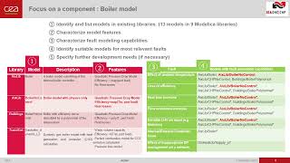
So here is the agenda for the presentation. I will talk first quickly about the way we simulated and generated the data, then a bit about the data set that we generated and then a bit more on the results with the machine learning models before a conclusion. Yes, so for the simulation model, as I mentioned, we simulate systems with folds. What we did is we used mostly open source models and mostly Modelica models for this simulation. So as a first step, what we did, we selected suitable models from the literature to do that. I won't go into details of the tables, but the first line shows you the.
Steps. So first we identified model, we characterized the model features. So we did a systematic review of a number of models. Then we linked that with the possible most relevant faults, which we also studied.
In different components we find in a district heating system. So that can be production components, the network itself and substation and storage components. And then we are identifying some of the well identified most suitable models for our purpose, with some minor modifications. So in the table there are underlined the models we chose and all the details go into the report from the project, which will be public. Okay, so let's go to the next slide. So for each of this model we perform simulation with the following principles. So at the center we have the simulation model, Modelica model in this case.
Which we simulate using. First, the two important thing to remember here is that we used boundary condition profiles of four weeks with a time step of one hour. And we have generated 13 of them corresponding to one year 52 weeks. So we have 13 different profiles. And for the simulation we generate random fault profiles with a fault pattern which is either a ramp or a step with a randomly chosen start time and intensity. So we have a number of possible simulations that we can run and we obtain results like on the right with of course different behavior depending whether it's normal or faulty situation. So on the right here we have the example I think on the fooling of a substation with the thermal heater. The conductance which is in blue is the reference one and the red is the one with a fault. Just to give you an idea of the simulations. Okay, so we can go to the next part.
So with that we generated full data set. So which I can show afterwards. The next part, next slide. Yeah, so this was inverted, but okay, can you go to the next one? Okay, so this was just a table summarizing all the simulation that we did. Of course I won't go into the details there, but we generated for several components with these profiles a number of random faults. So in total we obtained about 3 million recorded instance for the data set. So this is all saved in a CSV file and if you go one slide before. So I'm sorry, this was not the last version that I provided.
Sorry for that.
So this data set is available.
On the Kaggle platform which is online and open. So we provided the data set with all the metadata that is required to use it. If you notice, I made a screen capture of the page with a usability index of 10 out of 10. So we tried to make it as usable as possible and also included the IADHC logo with permission from the IADHC operating agent. And we have currently four data sets shared and also jupyter notebooks for usage examples. So this is ready to be used by all other people. So now I go to the last part of the presentation regarding the machine learning models. Unfortunately I won't be able to go go much into details on that, but I will give you just another view. Next slide. So first to. Yeah, just to maybe. Yeah, the one before. Just.
Yeah. So just to recap, there are several possible applications of machine learning for fall detection and predictive maintenance. This classification is taken from a paper, but there are many others like this. Here we are focusing only on the classification and binary classification.
Tasks which are supervised machine learning. So mostly we are trying to detect with binary classification whether there is a fault or no fault in a Specified simulation. And in terms of classification we have several tasks. I will talk quickly about it afterwards.
So yeah, next slide please. Okay, so regarding binary classification, so in that case we consider settings where we have simulations with either no fault or a given fault for given components. So here we have four components and five type of faults. So there can be only one fault at a time. So it's rather easy task. What we can see that. Well, we tested several machine learning algorithms. What we can see is that for some of the tasks, especially the one related to efficiency, while it's the machine learning models are picking up quite easily the faults. And it's more difficult with the task related to thermal losses. So heat losses in a boiler and insulation in a storage on the right. So of course there would be many details. I would just show you on the next slides a bit more detailed examples on a fault that can happen on the decrease of the COP of heat pump. So on the top we have an example with a strong decrease of the COP, so 84%. We can see that the COP, which is the gray line, is dropping. So this data is not available to the machine learning model. But from the other input data that we have, in that case the temperatures.
Temperatures, it can guess and find quite accurately the presence of a fault. And.
Looking at the graphs on the left, the orange points are depicting the fault detection probability which are rather close to zero at the beginning and go to one obviously when the fault is detected.
And on the right we have the fault detection after applying a filter to that. What is interesting is that on the second line we have the same example with very small and progressive cop decrease of 3%. And still in that case we can see that the model can pick and find that there is this fault. So the probability of a fault detection is increasing over time. And if we apply the filter, of course at the beginning we do not detect the fault, but after some time we can spot a fault on that. So that's interesting to see that it's possible, although visually we would not be able to find it. Okay, so maybe I will. Yeah, for the next slide.
So the next slide is about multiclass classification. So just to mention that we consider three types of tasks. One is to distinguish between different faults on one component. The other task is to distinguish on several possible locations for network leaks. And we also have one about different possible location for unbalance in a solar thermal field. But I won't go into detail there because I guess we don't have time. So probably we need to skip the next slide, which Was on the. On the leaks, on this small example. On the leaks and we go to the conclusion.
So for the goal of providing a reference data set, I've presented you well the overview of the data set we have, how we simulated it and how we provide it in the open data.
And for the assessment of the data set. So we implemented several type of machine learning models. So you have the list in the presentation and the details also in the. In the reports of the projects and the results I mentioned already are. Some tasks are well, easy to define, some are more difficult.
Some are more difficult and there can be interesting results for the leaks detection. Also something I did not.
Detail here is that we started to investigate all the models trained on the synthetic data set can transfer to a real system.
Which is a bit more complex to explain. But we're starting to do that and we will provide some results on that. Step further on maybe in other projects. Yes, thank you.
Okay, thank you very much. Matthieu. Sorry for not having shown the very last version of the presentation. Simon, very much. Thank you very much to you as well. If there are any questions in the audience, please just come up with them.
Was a bit dense I guess.
Maybe a question from my side. Is there any final report to read? If you want to, let's say to go through it a little bit more in detail maybe slowly.
Yes, of course we are just now we are creating the final report and I guess it will be ready in autumn or so. I'm not sure exactly but of course we do that and this will be public afterwards on the IEA website. Great.
May I ask one question?
Yeah, please.
So in the part that Simon was presenting, I was wondering if you. When you were considering the T set point based on the forecast and. And.
Step before. So what kind of T set point is. Were you referring to? Was associated to the aggregate then hitting demand and then the set point for the district network or if it's at the building level.
No, it's not the building level, it's the network level. I mean there's a. Currently there is already a control system in the DHN in Libano. So the set point is coming from this control, which is weather controlled. Which is weather controlled. Exactly.
And so then essentially it would be like providing a more accurate.
Assessment of what would be the set point in the network.
Yeah. In fact the point is that the current system is not taking into account really the latency time of the system. So this is sort of running right on the current demand, which is of course based on weather Forecast but also. Or outside temperature rather. But not really on the irradiation for example. And the point is that there's about 1.5 to 2 hours of latency in the network. That means this is not really accounted for. And by using such an AI approach you would much more be able to avoid especially overheating which is a problem in this kind of. When in the Lebanon district heating network. So that sometimes they're heating too much and they have to blow up or blow off. Sorry, not blow up, blow off the. The.
Vapor because they produce too much energy. So. Okay.
Okay, thank you.
Very interesting.
Yeah, thank you for this very condensed but very nice and compact information. Would be great to integrate the slides into our documentation if it's okay for you. Yeah, we just need the slides.
I would have a question on the first part on the forecasting regarding the. My. You have mentioned with citizen something percent I know.
Adaptive regression based methods which achieve lower mice even. Even though they are much simpler. Did you compare it to any other state of the art methods?
No, not really. You're completely right. I mean we should really do that in the future to check how it works. But. But the aim was really to check if these kind of methods are really able to. To do sort of a robust forecasting and regression analyst needs a lot of.
Yeah. Training as well and. Or parameterization.
Not if you do them in an adaptive manner then they are plug and play.
No, I mean you're right. It could be that conventional method is even better. This is completely right.
To provide the data. So the.
Heat flows and the ambient temperatures.
Yeah, we can check that. I mean you want to.
It would be interesting for me just to. To check it with other methods because then I get a better impression of this six point something.
Yeah, let's talk about that afterwards. How we could exchange the data.
Yeah. Would be great since we're a little bit overtime, but still. Okay, last question from Pakhtad.
Yes, thank you. Yeah, yeah.
A complete complimentary question to Marcus. Exactly. That was also my question because.
I.
Was wondering that if you have a.
Rough number of the features you've used.
For these ANN networks that you were using.
What do you mean by features?
The labels or.
The variables? The different variables that you.
Ah, okay. I mean this was the different temperature in the network at about how Many were there? 30 or 40 pressure temperatures at different points of the. Of the network and whether data input.
For the prediction models is only what is shown on. On one of the slides. So the first. The second one of my part.
Yes.
Where is it?
Or.
Still more.
This one.
This one.
Yeah, exactly.
So it's basically these four. I mean, the time is. Was encoded day of week.
Time of day and day of year, I think. And then additionally, global horizontal irradiance, ambient temperature and heat demand.
Okay.
Yeah.
Thank you.
Okay.
Since contact data are available, you may have a discussion later.
So.
Thank you. So I'm just.
Thank you. You're welcome.
Yeah, I'm just stopping the video.
More from IEA
XIV-05: Flexibility and DH value chain (FlexVal) – advanced analysis & compatible pricing
XIV-04: RE-PEAK - How to cover peak loads in district heating networks with renewables.

Digitalisation of District Heating: Summary of findings from IEA DHC Annex TS4
25/01/2024: The crucial role of district heating pipe lifespan in achieving climate objectives
IEA DHC XIII-03 Generation of simulated faulty datasets to ease heating network fault detection
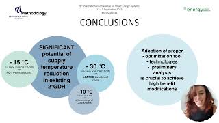
XIII-01: Leave 2nd generation behind: Cost-effective solutions for small to large scale DH networks
XIII-04: Cost Benefit study on the building secondary network for improving DH performance
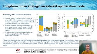
XIII-05: OPTiTRANS - Optimized transition towards low-temperature and low-carbon DH systems